Feel Tips - Fast Insert Excel Workbook Header or Footer to Every Sheet

A header or footer can be easily inserted to an Excel sheet through Excel’s Page Layout view. But when you need insert a same header to several or even all of the worksheets in Excel workbook, this could be a heavy repetitive work. However, you don’t have to insert a header or footer individually to every worksheet if you can group them. Continue reading this post, you will learn a fast solution to insert header or footer to every worksheet in workbook.

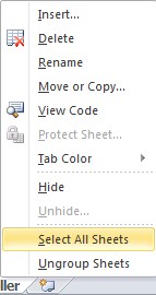
First, group all of the sheets. Right-click a sheet Tab and choose Select All Sheets from the resulting shortcut menu. It’s an easy trick for most Excel users to group all of the worksheets. 

Then, in the bottom-right, click the Page Layout button. Now we are in Page Layout view. Page Layout is new to Excel 2007. If you are using Excel 2003, you can choose Header and Footer from View menu.

Now you will find an area called “Click to add header” and you can enter your header there. The layout view supports the left, center, and right sections. Then, you can fully control the header at your will. If you want to display the sheet name, you can click Sheet Name in the same group. 

When you finish inserting header content, click any of the sheet tabs to remove the grouping. As you move from sheet to sheet, you’ll find that they all have the same header. This trick works inserting footers either. Here I want to give you all a friendly reminder. Headers or footers are visible only in Page Layout view and in Print Preview.

Wish this trick can save you a lot of time on your daily work. If you need repeat a task on multiple or all worksheets, you can group them together. 

Feel Tips - How to Customize Excel Sorting

Even though Microsoft Excel’s ascending and descending sort options are powerful tools, sorting in Excel is a common task. However, sometimes Excel doesn’t always sort values in a familiar and meaningful way. For example, when we sort months according to alphabetically, Excel might not sort in a meaningful way. According to the image below, we randomly enter 12 months in a column. After applying an ascending sort, the column list sorts alphabetically instead of sorting by month order.

When this is the case, we need a custom sort. Fortunately, Excel offers a custom sort. In Excel 2003, just follow the steps below. 

1. Select the month names. In this case of the above image, that’s A2:A13.

2. Choose Sort from the Data menu.

3. The resulting dialog box anticipates the custom sort. The Sort By control displays Month with an Ascending sort. If you click OK, Excel will sort the selected months in alphabetic order.

4. Click the Options button at the bottom of the dialog box. 

5. In the resulting dialog box, the First Key Sort Order control displays Month. Click the dropdown arrow to display four custom sort options.

6. Choose the last option, January, February, March, and so on. By default, a custom sort isn’t case-sensitive, but there’s an option to make it so, if you need it.

7. Click OK twice and Excel sorts the months in the familiar way you expect.

In Excel 2007 and 2010, there’s a little different:

1. Click the Sort option in the Sort & Filter group. (Don’t click the A to Z or Z to A sort icons, the ones with the arrows.)

2. In the resulting Sort dialog box, click the Order control’s dropdown list and choose the appropriate custom sort.

3. Click OK.

Custom sorting in Excel, the list doesn’t have to contain all of the sort elements to work. A list of a few months can still sort by month order.  

Feel Tips - Create a Custom Sort in Excel

Learn how to create a custom sort for unique sorting needs that alphabetic and numeric sorts just can’t handle.

In the last article “How to Custom Sort in Excel” we discussed special sorting solutions which don’t follow alphabetic and numeric order. There are four of these special sorting solutions built-in Excel custom sorts. For most of time, they are not enough. Fortunately, Excel enables you to create a custom sort if it’s necessary. For example, if you want to identify temperatures by Cold, Warm and Hot, but alphabetic sort would make it by Cold, Hot and Warm. However, you can create a custom sort to make it sort as your wish.

Now, let’s create a custom sort in this case of temperature. In Excel 2010, just follow the steps below: 

1. Go to the File tab and select Options (under Help).

2. In the left pane, select Advanced.

3. In the General section, click Edit Custom Lists.

4. After we are in List Entries control, enter each element in the sort order as you wish. Press Enter after each entry. (If the list is long or already exists as natural data, you can specify the cell reference and click Import). 

5. Click button Add, as the image shows below, Excel will transfer the new custom sort order to the Custom Lists control (on the left).   

6. After that Click OK twice.

In Excel 2007, there is a bit different:

1. Click the Office button and click Excel Options.
2. In the left pane, click Popular (the default).
3. In the Top Options For Working With Excel section, click the Edit Custom Lists button.
4. Continue with step 4 above in Excel 2010.

To apply the custom sort, select the list you want to sort, click the Data tab, and then click Sort in the Sort & Filter group. Click the Order dropdown, choose Custom Lists, and select the Cold, Warm, Hot list.

If you are using Excel 2003, you can create custom sort by following the steps below:

1. Go to Options from the Tools menu.
2. Click the Custom Lists tab.
3. Continue with step 4 above in Excel 2010.

To apply the custom sort in Excel 2003, select the list, and choose Sort from the Data menu. Click the Options button, choose the custom sort from the First Key Sort Order dropdown, and click OK twice.

When you create a custom sort list, it’s not just for the one you are working but for all workbooks. Custom lists are stored in the Windows Registry which means it can’t be used on other computers. However, if you’re working with the same workbook, the list itself is available. If you want to add the created new custom sort to a local system’s registry, you can open the Custom Lists dialog box, select the list in the Custom Lists control and click button Add. 

Feel Tips - Copy or Move Excel Worksheet from One Workbook to Another

What will you do if you have to copy or move a worksheet data from one workbook to another? It sounds like a complicated job. In truth, we can easily copy the whole Excel worksheet and paste into another workbook. Excel has a built-in feature that makes quick work of this task, but as usual, there’s more than one way to get the job done in Excel.

Solution 1 Copy or Move Worksheet via Excel User Interface

First, open both the source and the target workbook. Go to the source workbook and navigate the worksheet which we want to copy or move. Then, click Home tab and then click the Format dropdown in the Cells group. Select “Move or Copy Sheet” in the Organize Sheets section as the image shows in the below. In edition 2003, we can select “Move or Copy Sheet” from Edit menu. 

Now, in the “Move or Copy Sheet” dialog, select the target sheet from the To Book dropdown. Excel will display only the open workbooks in this list. Here we can also update the Before Sheet selection.

If we want to copy rather than move the worksheet, click the Create a copy option at the bottom of the dialog. Click OK and Excel will copy or move the worksheet to the target workbook.

Solution 2 Copy or Move Worksheet via View Menu

First, open both the source and target workbooks. Then, follow the simple 2 steps below:

1. Go to the View tab and choose View Side By Side in the Window group. Excel will split the screen, horizontally, between the two workbooks. In Excel 2003, you’ll find this option on the Window menu.
2. Click the sheet tab in the source workbook and drag it to the target workbook. If you want to copy the sheet instead of move it, hold down the [Ctrl] key while you drag the sheet to the target workbook.

That’s all there is to it! The next time you need to copy or move worksheet data from one workbook to another just drag the worksheet.

Friendly Reminder: if the source worksheet contains a procedure that references another sheet in the source workbook, Excel will do its best to find the source workbook. If it can’t, when you run that procedure, you will get errors. 

Feel Tips - Compare Columns of Excel Data with a Quicker Way

Microsoft Excel is the most popular application for users to handle different data information. Sometimes we need compare data in worksheet. Microsoft Excel offers a number of ways to compare data. For instance, conditional formatting is an easy way to highlight differences as they occur. However, if you don’t need a dynamic and more permanent solution, there is a quicker way.

In this post, you will learn a little-known feature in Excel which can quickly compare one or more columns of data to another. Now, follow the steps below to work through a simple example. 

1. Select the multi-column data in Excel worksheet. This solution works with one or more columns. It’s important to remember that the feature compares all selected columns to the first column in the selection (as anchored, which isn’t necessarily the left-most column). In this case, you’d select cells A27:C27 (see below).

2. Press [F5] to launch the Go To dialog.

3. Click the Special button at the bottom as the image shows.

4. In the resulting dialog, select Row Differences.

5. Click OK and Excel highlights the values in columns B and C that don’t match their corresponding values in column A.

In step 1, I mentioned anchoring. If you anchor the selection by selecting from the last cell in the right-most column and then highlighting from right to left, Excel will compare values in columns B and A to the values in column C.

It's temporary to compare columns of Excel data by using this solution. But if you just need one-time comparison, this should be a quicker and easier way to find differences between columns.

Feel Tips - Fast Find Excel's XLStart Folder

When you install Microsoft Excel, a special fold XLStart will be created. XLStart folder is a place for Excel to store the workbook template, Book.xltx. If we store a workbook in XLStart folder, Excel will open it when we launch Excel  automatically at every time.

However, users seldom use the XLStart folder. When we want to use XLStart folder in a special time we might not remember the entire path. So XLStart folder is difficult for us to find it out. In addition, the location isn’t always the same from system to system (it depends on your operating system and other installation priorities). When sometimes, we need to update the workbook template or save a workbook to XLSStart folder, we may never find it. Even we find it at last it may cost us a lot of time.

Fortunately, there is a quick solution to find Excel’s XLStart folder. Through Immediate Window in the VBE (Visual Basic Editor) we can fast find Excel’s XLStart folder.Follow the steps below:

1. Open an ExcelWorksheet
2. Press [Alt]+[F11] to launch the VBE.
3. If the Immediate Window isn’t visible, press [Ctrl]+g.
4. In the Immediate Window, type ? application.StartupPath and press key Enter. VBA will display the path to XLStart.

Wish this quick Excel tip can help you at some time when you need find Excel’s XLStart folder. 

Customize Excel Default Settings to Work as Your Way

People are different. They have different requirements. So, the out-of-the box environment of Microsoft Excel might not provide the most efficient setup for you. When you create a new workbook, if you find yourself changing the same attributes every time, you can consider changing them at the program or template level. Customize Excel default settings, Excel will generate each new workbook just the way you like it. Sometimes, changing some default settings to meet your needs can save you tons of time and make you happy on working. There are some samples that many users customize to meet their needs. Maybe you can find some good for you. 

1. File Location

The Excel default file location is “My Documents”. You can quickly customize this default setting as follows:

1. Go to the File tab and choose Options (under Help). In Excel 2007, go to the Office button and then click Excel Options. In Excel 2003, choose Options from the Tools menu.
2. In the left pane, choose Save. In Excel 2003, click the General tab.
3. In the Save Documents section, change the path in the Default File Location field, as shown in the image below. You can type the path or click Browse to locate it.
4. Click OK.

2. Number of sheets

In the Excel default setting, each new workbook includes three sheets. You can easily add or delete sheets, but you can also change the number of default sheets, as follows:

1. Go to the File tab and then click Options (under Help). In Excel 2007, click the Office button and then click Excel Options. In Excel 2003, choose Options from the Tools menu.
2. Click General in the left pane. In Excel 2003, click the General tab.
3. In the section of When creating new workbooks, enter the number of sheets in the Include this many sheets field, as shown in image below. In Excel 2003, use the Sheets in new workbook drop-down.
4. Click OK.

3. Open a Specific Workbook

If you often work with the same workbook, it can save some time by opening a specific workbook when launching Excel. This shortcut is easily accomplished by saving that workbook in the XLStart folder. Depending on your version of Windows, you’ll find that folder in one of the following locations:

• Windows XP: C:\Documents and Settings\user name\Application Data\Microsoft\Excel\XLStart
• Windows Vista: C:\Users\user name\AppData\Local\Microsoft\Excel\XLStart
• Windows 7: C:\Program Files\Microsoft Office\Office\XLStart

Just save the workbook as you normally would, but save it to the appropriate XLStart folder.

4. Cursor Movement

In Excel worksheet, when you press “Enter”, Excel moves the cursor down one cell. But if you want to enter data by moving to the right, rather than down, you may want to change the cursor movement, as follows:

1. Go to the File tab and then click Options (under Help). In Excel 2007, go to the Office button and then click Excel Options. In Excel 2003, choose Options from the Tools menu.
2. In the left pane, select Advanced. In Excel 2003, click the Edit tab.
3. In the Editing Options section, choose Right from the Direction drop-down under the After Pressing Enter, Move Selection option, as shown in the image below. You can choose Right, Left, Up, and Down. In Excel 2003, the option is Move selection after Enter. Uncheck the option can stop cursor movement.
4. Click OK.

5. Font and Size

The default setting of Excel font and size can also be customized. By doing so, you eliminate the task of adjusting each new workbook. To change the default font, do the following:

1. Go to the File tab and then click Options (under Help). In Excel 2007, click the Office button and then click Excel Options. In Excel 2003, choose Options from the Tools menu.
2. Choose General (if necessary) from the left pane. In Excel 2003, click the General tab.
3. In the When Creating New Workbooks section, change the Use This Font (Standard Font in Excel 2003) and Font Size options, as shown in the image below.
4. Click OK.

6. Template

Like Word, Excel bases each new workbook on a template file (Book.xltx) which can be permanently changed by adjusting many default settings. You can make this change once to Book.xltx, instead of adjusting each new workbook manually.

When making changes at the template level, you can start in one of two ways:

• If you’ve customized Book.xltx, open it so you don’t lose prior changes.
• If you haven’t customized Book.xltx, you can begin with any blank workbook.

Make the changes you want to implement at the template level and then save the workbook as a template:

1. Go to the File tab and choose Save As. In Excel 2007, click the Office button and choose Save As. In Excel 2003, choose Save As from the File menu.
2. Choose Excel Template (.xltx) from the Save As Type drop-down, as shown in the image below. Excel 2003’s template extension is .xlt.
3. Locate the XLStart folder using the Save In control. You must save Book.xltx to the XLStart folder.
4. Click Save.

If you can’t find XLStart, you can use Excel’s Visual Basic Editor to find the path, as follows:

1. Launch Excel’s VBE by pressing “Alt + F11”.
2. If the Immediate window isn’t visible, press Ctrl + G.
3. In the Immediate window, type ? application.StartupPath and press Enter, as shown in the image below.

If you want to alter things at the sheet level, make your changes and save the file as Sheet.xltx. You’ll use this file to change things such as inhibiting gridlines.

7. Startup folder

Tips #3 and #6 both rely on the XLStart folder to open or use specific files when you launch Excel. However, you can add a second location as follows:

1. Go to the File tab and then click Options (under Help). In Excel 2007, go to the Office button and then click Excel Options. In Excel 2003, choose Options from the Tools menu.
2. Choose Advanced in the left pane. In Excel 2003, click the General tab.
3. In the General section, enter the path to the new alternate startup folder, as shown in the image below.
4. Click OK.

Excel will continue to open any workbooks found in XLStart, in addition to those workbooks found in the alternate startup location.

8. File format

Many organizations must deal with version compatibility issues because some users upgraded to the Ribbon version before others. When sharing Excel 2007 and 2010 files (.xlsx format) with Excel 2003 users, you must downgrade the workbook to the older format (.xls). Doing so is no big deal, but if you have to do it for every workbook, you might as well change the default file format to .xls, as follows:

1. Go to the File tab and choose Options (under Help). In Excel 2007, go to the Office button and then click Excel Options.
2. Choose Save in the left pane.
3. In the Save Workbooks section, choose Excel 97-2003 Workbook (*.xls) from the Save Files in This Format drop-down, as shown in the image below.
4. Click OK.

However, by using this method, we can’t use new features. Download and install the compatibility pack might be much easier.  

9. Enable Text Wrap

When we enter a long string into a cell, Excel allows it to extend past the column’s right border. If there’s no data in the adjacent cells, the entire string is visible. But once you enter data in the adjacent cell, the new data takes precedent and the original string disappears behind the new text. This happens at the format level and we can reset this alignment attribute by adjusting the Normal style. Unfortunately, that doesn’t help all the other workbooks you create. If this is a format you want to set for all new workbooks, change the Normal style in book.xltx (#6):

1. Go to the Home tab. Then, in the Styles group, click the Cell Styles drop-down. In Excel 2003, choose Style from the Format menu.
2. In the resulting gallery, right-click Normal and choose Modify, as shown in the image below. In Excel 2003, select Normal in the Style Name control, click Modify, and then skip to step 4.

3. In the Style dialog, click Format.

4. Click the Alignment tab and select the Wrap Text option in the Text Control section, shown in the image below.

5. Click OK twice.

Changing the Normal style only works in the current workbook. For all new workbooks, you need to save at the template level to adjust the style.

10. Comment Font Size

To customize Excel comment font size would take a detour from the traditional routes. We must change a Windows setting.

For Windows XP, do the following:

1. Right-click the desktop and choose Properties.
2. Click the Appearance tab and then click Advanced.
3. From the Item drop-down, choose ToolTip.
4. Select a font size and click OK.
5. Click Apply and then click OK.

Windows 7 users should do the following:

1. Right-click the desktop and choose Personalize.
2. Click Window Color.
3. Click Advanced Appearance Settings.
4. From the Item drop-down, choose ToolTip.
5. Choose a font size.
6. Click OK and then click Save Changes.

This change will update all tip-type windows, not just Excel comments. So be sure you can live with the total package, especially if you share your system with other users.

Note: Although the dialog will let you specify a different font, Excel will ignore the new setting.

Feel Tips - Control Excel Cursor Movement during Data Entry

Data entry is a usual job when we work with Excel spreadsheet. If we can control Excel cursor movement during data entry, this job can be a thankless job, or else it can be a hateful job. In this post you will be introduced some quick tips for controlling cursor’s movement.

First, change cursor movement setup

You can easily press key “Enter” to move the cursor down to the next cell. Or if you are entering data from column to column you can press “Right Arrow Key”.  Perhaps press key “Tab” is easier. However, the easiest solution is to change the cursor movement setup as the following steps.

1. Click “File” tab to “Options (under Help)”. In Excel 2007, click the “Office” button, and then click “Excel Options”. In Excel 2003, choose “Options” from the “Tools” menu.
2. In the left pane, select “Advanced”. In Excel 2003, click the “Edit” tab.
3. In the “Editing Options” section, select “Right” from the Direction dropdown under the After Pressing Enter, Move Selection option, as shown. You can choose Right, Left, Up, and Down. In Excel 2003, the option is Move Selection After Enter.
4. Click OK.

This can make your data entry job at your will from the beginning. If you don’t like the style, it’s easy to reset.

Second, select data input range

This trick is a temporary solution. Before enter data, we can select the data input range. Excel will move the cursor from column to column until you reach the right-most column in the selection. When we press key “Enter”, the cursor will be moved to the left-most column in the next row. For example, if we want to enter data in A29:B33 as the image shows below, we can first select the area. When we input data, Excel will automatically select A29. After that will be B29. And then, it’s A30 not C29.

Third, table feature in Excel

The table feature of Excel can simply convert input range to a table. In a table, Excel will control data input as trick 2. Create table in Excel can be very easy by follow the steps below (Excel 2003 doesn’t support Table feature).

1. Click the “Insert” tab.
2. In the Tables group, click “Table”.
3. Specify whether the range has header cells or not, and click OK.

Now, you don’t have to do anything but starting data entry.

Wish these tricks for controlling cursor movement can make your data entry job with happiness. 

Feel Tips - Transpose Data from Rows to Columns in Excel

When you deal with data in an Excel worksheet, you can always find some easy way.  For example, when you want to transpose data from rows to columns, you don’t need to do it manually. Microsoft Excel provides a handy transpose option that will quickly take care of the task.

Suppose we’ve put some data information in an Excel worksheet. There are three column headings running across Row 1 and four row headings running down Column A. Details can be found in the image below.

Now, if we want to transpose data from rows to columns, we don’t have to re-key the data to make the current set of row labels (months) running across the columns.

First, select and copy the entire data range. Then, choose a location in the worksheet to place data. Third, right click to Paste Special menu. A new window will pop up.  Fourth, select the checkbox as the image below (transpose-data-2). At last, click OK. The data will be transposed from rows to columns automatically. 

Result Effect:

Through Past Special menu, you are not limited to transpose data from rows to columns. It works as well when you need to turn a single row of labels into a column, or vice versa.